DoRA Demystified: Visualising Weight-Decomposed Low-Rank Adaptation

Unlocking DoRA's Mechanisms: Reproducing Research Paper Results to Explore Its Inner Workings

This work is inspired from

Sebastian Raschka, PhD

blog on LoRA and DoRA from scratch.

Fine-Tuning allows us to leverage existing pre-trained foundation models and adapt them to specific tasks or domains. By training the model on domain-specific data, we can tailor it to perform well on targeted downstream tasks. However, this process can be resource-intensive and costly, as we will be modifying all the millions of parameters, as part of training. Fine tuning the model requires a lot of training data, huge infrastructure and effort.

Applying complete fine-tuning to a single model for different domain-specific tasks often results in creating large models tailored to specific tasks, lacking modularity. We need a modular approach that avoids altering all parameters, while demanding fewer infrastructure resources and less data.

Low-Rank Adaptation (LoRA) is a PEFT method that decomposes a large matrix into two smaller low-rank matrices in the attention layers. This drastically reduces the number of parameters that needs to be fine-tuned.

DoRA is another novel PEFT method that incorporates weight decomposition by using magnitude and directional components of weight vectors, achieving a learning capacity closely resembling full finetuning (FT) without any additional inference latency over LoRA.

Average accuracy of LoRA and DoRA for varying ranks (annotated figure from the DoRA paper: https://arxiv.org/abs/2402.09353)

From the above figure, we can observe that DoRA has consistently surpassed LoRA across all ranks below 8. DoRA quality is superior to LoRA especially in lower ranks. The difference in quality of DoRA of rank 8 and LoRA of rank 8 appears to be more significant than training ranks of 32 or 64.

Hyper parameter Configuration

I reproduced the visualizations for magnitude and directional components of query and value weight matrices for LoRA and DoRA adapters using Llama-2-7B-hf pretrained LLM as shown in the (DoRA paper). These results correspond to finetuning the pretrained LLM for cleaned alpaca Instruction dataset. The hyper parameters for finetuning used here are same as those mentioned in Appendix section of DoRA paper.

Adding LoRA adapter weights to foundational model introduces two new matrices of smaller dimension (matrix A and matrix B). Pretrained model weights are frozen (non-trainable) and only the adapter LoRA weights are learnt during finetuning process. For below hyper parameter combination, the number of trainable parameters accounts to only 2.31% of total number of parameters. This would enable faster training with lesser compute or hardware requirements.

peft_config = LoraConfig(
    r=64,
    lora_alpha=128,
    lora_dropout=0.0,
    target_modules=["q_proj", "k_proj", 
"v_proj", "o_proj", "gate_proj", "up_proj", "down_proj"],
    bias="none",
    task_type="CAUSAL_LM",
    inference_mode=False
)

model = get_peft_model(model, peft_config)
model.print_trainable_parameters()

All Parameters: 6,898,323,456 || Trainable Parameters: 159,907,840 || Trainable Param %: 2.3180681656919973

Now let’s check the total trainable parameters for DoRA adapter. By setting use_dora=True in LoraConfig, DoRA weights are added into the foundational model. Using same hyperparameter setting as above, it can be observed, total trainable parameters increased marginally from 2.318% to 2.337% (~0.02%). In DoRA, LoRA weights are decomposed into magnitude and directional components. The magnitude vector is trainable. Directional component is taken care by LoRA weights. This is the reason behind marginal increase in trainable parameters as shown below.

peft_config = LoraConfig(
    use_dora=True,
    r=64,
    lora_alpha=128,
    lora_dropout=0.0,
    target_modules=["q_proj", "k_proj",
 "v_proj", "o_proj", "gate_proj", "up_proj", "down_proj"],
    bias="none",
    task_type="CAUSAL_LM",
    inference_mode=False
)

model = get_peft_model(model, peft_config)
model.print_trainable_parameters()

All Parameters: 6,899,683,328 || Trainable Parameters: 161,267,712 || Trainable Param %: 2.337320487529482

Now, let’s check if the DoRA layers have been added as expected in the foundational model. As the rank is set to 64, the LoRA matrices A and B are decomposed into (64, 4096) and (4096, 64). The magnitude vector is computed along the column dimension of pretrained weight matrix. Hence it’s shape is 4096.

for module in peft_model.model.model.layers:
    print(module.self_attn.q_proj.weight.shape)
    print(module.self_attn.q_proj.lora_A.default.weight.shape)
    print(module.self_attn.q_proj.lora_B.default.weight.shape)
    print(module.self_attn.q_proj.lora_magnitude_vector)
    break

Shape of Pre-trained Query Weight Matrix -> torch.Size([4096, 4096])
Shape of LoRA - A matrix for Query Weight -> torch.Size([64, 4096])
Shape of LoRA - B matrix for Query Weight -> torch.Size([4096, 64])
Trainable Magnitude Vector -> ParameterDict(  (default): Parameter containing: [torch.cuda.FloatTensor of size 4096 (cuda:0)])

By using above configuration, the PEFT model is finetuned with LoRA and DoRA adapters for 1 epoch on cleaned alpaca instruction dataset. For every 100 training steps, checkpoints for adapter weights are stored. These checkpoints are later utilized to visualise the Magnitude and Directional changes happened from pretrained model weights to finetuned adapter weights. Now, let’s jump into the most interesting part of this blog.

Weight Decomposition Analysis

Once the model has been finetuned for LoRA and DoRA with checkpoints stored for intermediate training steps, Let’s start analysing the weights

I’ll break down this section into following steps:

1. Load the model weights for query or value weight matrix for each decoder layer in foundational model (32 decoder layers)

2. Merge the LoRA matrices (A and B) for each query or value weight matrix in the decoder layer with it’s corresponding pretrained weights.

3. Merge the DoRA adapter weights with pretrained weights for each linear layer and load the corresponding query or value weight matrix.

4. Decompose the pretrained, merged LoRA and merged DoRA weights into it’s magnitude and directional components and store it for further computations

5. Compute the change in magnitude and directional components of pretrained and merged LoRA weights and repeat the same for merged DoRA weights

6. Repeat from step 2 to step 5 for every checkpoint stored while finetuning process

7. Combine the magnitude and direction values in a dictionary for visualization

Below code is used to merge the LoRA weights with pretrained weight matrices. Query or Value weights are stored in a list for pretrained, LoRA and DoRA models.

def merged_lora_weights(layer):
    alpha = 2 * layer.lora_A.default.weight.shape[0]
    lora_weights=layer.lora_A.default.weight@layer.lora_B.default.weight
    combined_weights = layer.base_layer.weight + alpha*lora_weights
    return combined_weights

def get_model_weights(model, tag='pretrained'):
    query_weights = []
    if tag != 'dora':
        for layer in model.model.model.layers:
            if tag == 'pretrained':
                query_weights.append(
                    layer.self_attn.q_proj.base_layer.weight
                    )
            if tag == 'lora':
                query_weights.append(
                    merged_lora_weights(layer.self_attn.q_proj)
                    )
    else:
        for layer in model.model.layers:
            query_weights.append(layer.self_attn.q_proj.weight)
    return query_weights

The magnitude and directional variations between pretrained weights (W₀) and finetuned weights (W_ft) is defined as below. In this article, finetuned weights are referred to LoRA or DoRA adapter weights.

\(\Delta M_{FT}^{t} = \frac{1}{k} \sum_{n=1}^{k} |m_{FT} ^{n,t}- m_{0}^n|\)

\(\Delta D_{FT}^{t} = \frac{1}{k} \sum_{n=1}^{k} (1 - cos(V_{FT}^{n,t}, W_{0}^n)) \)

Here, cos(. , .) represents cosine similarity function. V_ft {n, t} and Wo {n} are nth columns in V_ft {t} and Wo. Above equations represent the code written below for delta_magnitude and delta_direction

def weight_decomposition(weights, store: dict, tag=None):
    for i in range(len(weights)):
        magnitude = weights[i].norm(p=2, dim=1, keepdim=True)
        direction = weights[i] / magnitude
        store[f"query_layer_{i}"].append(magnitude)
        store[f"query_layer_{i}"].append(direction)

def cosine_similarity(a: torch.tensor, b: torch.tensor, dim: int):
    dot_product = torch.sum(a * b, dim=dim)
    norm_A = torch.norm(a, dim=dim)
    norm_B = torch.norm(b, dim=dim)
    sim = dot_product / (norm_A * norm_B)
    return sim


def delta_magnitude(pt_weights, ft_weights):
    layer_wise_delta_m = {}
    for i in range(layer_start, layer_end):
        a = ft_weights.get(f"query_layer_{i}")[0]
        b = pt_weights.get(f"query_layer_{i}")[0]
        k = b.shape[0]
        d_m = torch.sum(abs(a - b)) / k
        layer_wise_delta_m[f"layer_{i}"] = round(d_m.item(), 6)
    return layer_wise_delta_m


def delta_direction(pt_weights, ft_weights):
    layer_wise_delta_d = {}
    for i in range(layer_start, layer_end):
        a = ft_weights.get(f"query_layer_{i}")[1]
        b = pt_weights.get(f"query_layer_{i}")[1]
        k = b.shape[0]
        sim = cosine_similarity(a, b, dim=0)
        d_m = torch.sum(1 - sim) / k
        layer_wise_delta_d[f"layer_{i}"] = round(d_m.item(), 6)
    return layer_wise_delta_d

Around 5 checkpoints from five different training steps are considered for analysis. It comprises four intermediate steps and the final checkpoint from both LoRA and DoRA adapters. A weight decomposition analysis on each of these checkpoints is performed to determine delta magnitude and delta direction across different layers.

def get_magnitude_directions(tag):
    checkpoint_path = f"trl/output/{tag}"
    artifacts = os.listdir(checkpoint_path)
    combined_dm, combined_dd = defaultdict(list), defaultdict(list)

    for model_dir in artifacts:
        decomposed_weights = defaultdict(list)
        model_path = os.path.join(checkpoint_path, model_dir)
        new_model = PeftModel.from_pretrained(model, model_path)
        query_weights = get_model_weights(new_model, tag=tag)
        del new_model

        weight_decomposition(query_weights, decomposed_weights, tag=tag)
        dm=delta_magnitude(pretrained_weight_decomp, decomposed_weights)
        dd=delta_direction(pretrained_weight_decomp, decomposed_weights)

        name = model_dir[-3:]
        combined_dm[name].append(dm)
        combined_dd[name].append(dd)
    return combined_dm, combined_dd

Combine the magintude and direction and store it according to each layer across different checkpoints. This is just done to plot the below figures.

checkpoint_wise = []
for model_name in ['300', '400', '500', '600', '700']:
    if model_name in lora_m and model_name in lora_d:
        magnitude, direction = lora_m[model_name], lora_d[model_name]
        layer_wise = {}
        for m, d in zip(magnitude[0].items(), direction[0].items()):
            layer_wise[m[0]] = {"magnitude": m[1], "direction": d[1]}
        checkpoint_wise.append(layer_wise_magnitude_direction)

print(f"Checkpoint Wise Magnitude and Direction ->{checkpoint_wise[0]}")

Checkpoint Wise Magnitude and Direction -> 
{
'layer_1': {'magnitude': 5.398438, 'direction': 0.705566}, 
'layer_2': {'magnitude': 4.851562, 'direction': 0.681641},
...... upto layer_n
}

The full code example is available in my GitHub repo here: https://github.com/shreyassks/DoRA

Visualizing Magnitude and Directional Components

Magnitude and Direction updates for LoRA and DoRA for query and value matrices across different layers of decoder layer and intermediate steps are shown below. Different markers represent matrices of different training steps and different colors reperesent the matrices of each layer.

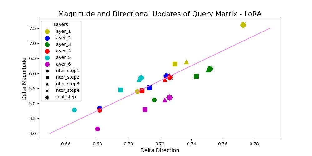
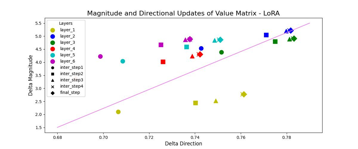
From above figures for LoRA, it can be clearly observed that LoRA tends to either increase or decrease the magnitude and direction updates proportionally. LoRA doesn’t have the capability to make small directional changes with more significant alterations in the magnitude or viceversa. A positive correlation is observed with a value of 93% and 84% for Query and Value matrices respectively.

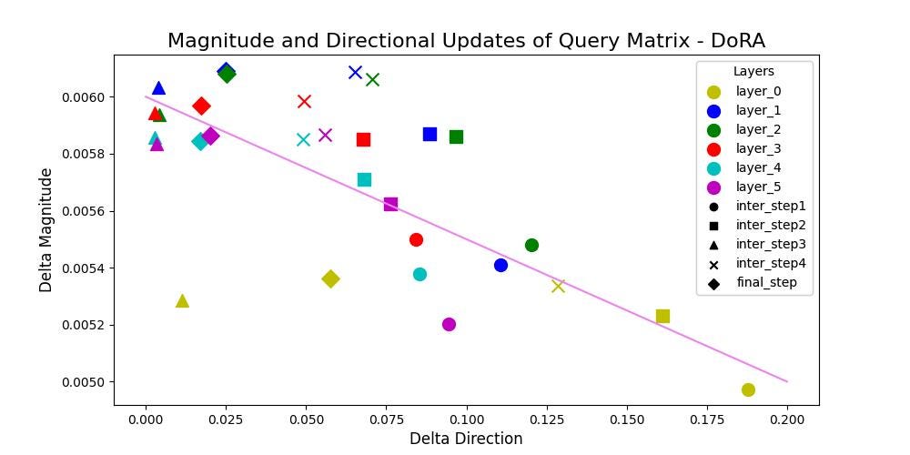
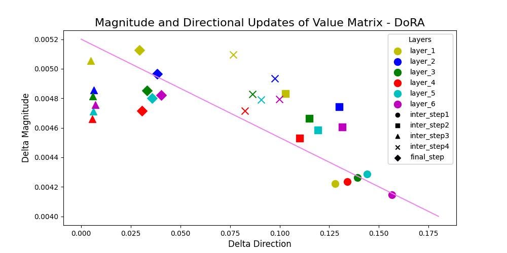
From above figures for DoRA, it can be concluded that DoRA demonstrates the ability to make only substantial directional changes or adjustments with minimal updates in magnitude or viceversa. A negative correlation is observed with a value of -62% and -69% for Query and Value matrices respectively.

Conclusion

It can be concluded that, DoRA can easily adapt on downstream tasks using very lower rank matrices compared to that of LoRA. DoRA finetuned weight update patterns resemble very closely to that of fully finetuned model without adding any additional inference latency over LoRA. This signifies that, when provided with adequate learning capacity, either having larger magnitude or directional updates itself is sufficient enough for adapting on downstream tasks. LoRA’s updates showed positive correlation of 93% and 84% for Query and Value matrices respectively, whereas DoRA’s updates showed a negative correlation of -62% and -69% for Query and Value matrices respectively.